Parent Vectors#
At the end of the previous section we settled on the parent vector representation as the main representation of trees we will be using in this tutorial. To reiterate, to represent a tree of \(n\) nodes, we associate each node with an index in ⍳n, and create an \(n\)-element vector parent such that if a node i is a child of a node j, then parent[i]=j.
We’re going to use a slightly larger tree for the examples in this section:
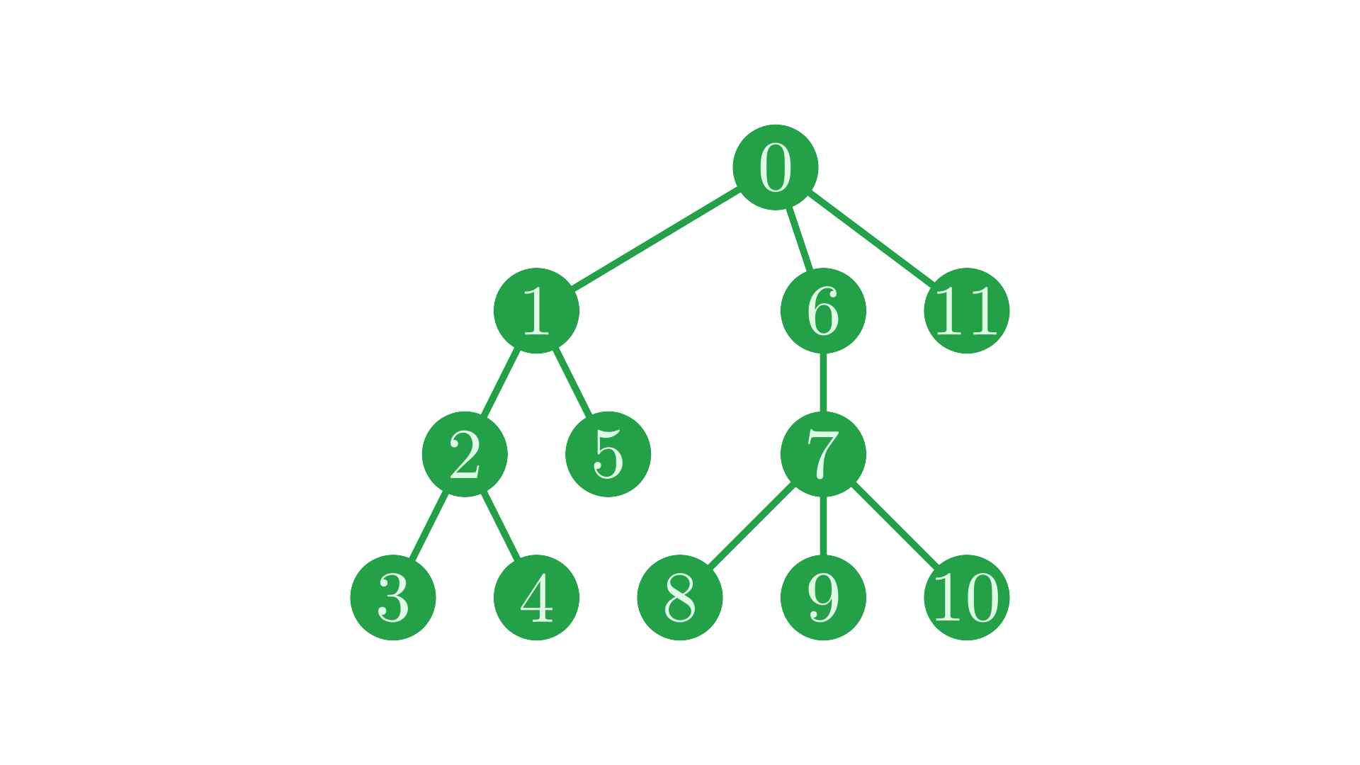
Fig. 9 The tree we’re going to work with in this section.#
and the parent vector representing this tree:
⊢parent←0 0 1 2 2 1 0 6 7 7 7 0
0 0 1 2 2 1 0 6 7 7 7 0
        ┌───────────┐─────────┐
        ┌─┐ ┌─┐─┐   │ ┌─┐─┐─┐ │
        ↓ │ ↓ │ │   │ ↓ │ │ │ │
parent: 0 0 1 2 2 1 0 6 7 7 7 0
          ↑ │     │ ↑ │
          └─┘─────┘ └─┘
In this section, we’re going to look at some of the basic operations you can do on trees represented in this way.
Basic Operations#
For brevity, we’ll abbreviate parent to p from now on.
p←parent
Finding Children#
Given a node i, the children of i are all those nodes whose parent is i. We can therefore easily create a mask of nodes which are children of i:
i←1
p=i    ⍝ nodes 2 and 5 are children of node 1
0 0 1 0 0 1 0 0 0 0 0 0
If we have multiple nodes which we want to find the children of, we can simply mask for those nodes which have a parent that is any of the parent nodes in question:
i←1 6
p∊i    ⍝ additionally, node 7 is a child of node 6
0 0 1 0 0 1 0 1 0 0 0 0
Applying ⍸ gives us the nodes which this mask selects.
⍸p∊i
2 5 7
Finding Leaves#
We can create a vector of all the node IDs in a tree, as it is just every index in p.
⍳≢p
0 1 2 3 4 5 6 7 8 9 10 11
The leaf nodes are those nodes which do not have any children, i.e. those nodes which are not pointed to in the parent vector. We can think of the parent vector as a list of all nodes which are not leaves, and remove them from a list of all nodes to obtain only the leaf nodes:
(⍳≢p)~p
3 4 5 8 9 10 11
Alternatively, if we want a mask of leaf nodes, we just mask those nodes which are not in the parent vector:
~(⍳≢p)∊p
0 0 0 1 1 1 0 0 1 1 1 1
Trimming Branches#
Time for our first structural change to a tree. Say that we want to remove a sub-tree from the main tree, but still keep the nodes around for reference. In a sense, we just want to snip the connection between a parent and child node:

Fig. 10 Trimming the branch between nodes \(0\) and \(6\).#
Recall that a root node (a node with no parent) is indicated by a self-loop in the parent vector - it is considered its own parent. Because of this, it’s easy to trim a node from its parent by setting its parent to itself.
i←6
i@i⊢p     ⍝ using @
p[i]←i    ⍝ using indexing
p
0 0 1 2 2 1 6 6 7 7 7 0
0 0 1 2 2 1 6 6 7 7 7 0
Note that the above code also works when given a vector of indices to be trimmed off, instead of a single scalar index.
Interestingly, p now represents two disconnected trees. The parent vector representation is versatile enough to handle this.
Finding Roots#
Given a parent vector which represents multiple trees, we may like to find which tree each node is part of. Each tree is uniquely identified by its root node, so we can find the tree each node is a member of by finding which root node it descends from.
After trimming node \(4\) from our tree, our two new trees look like:
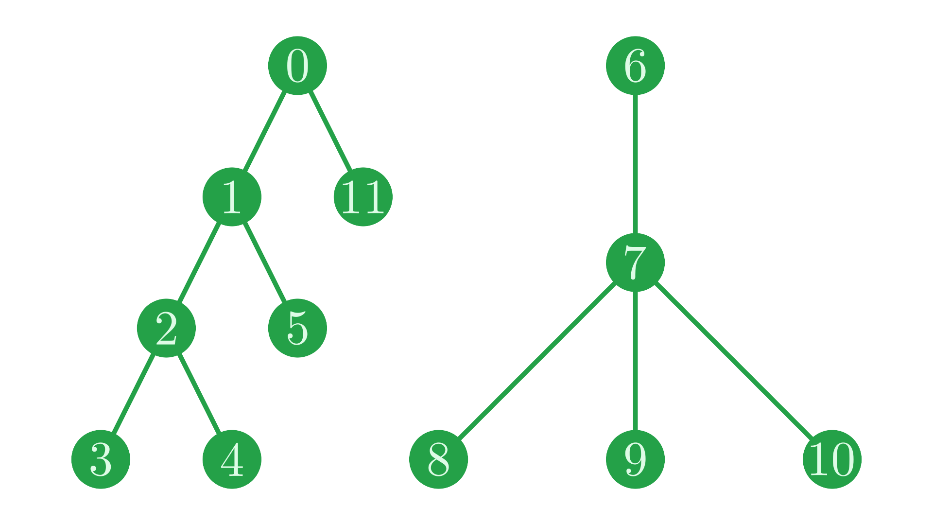
Fig. 11 Our two trees after snipping the branch between nodes \(0\) and \(6\).#
and they are represented by the parent vector:
        ┌─────────────────────┐
        ┌─┐ ┌─┐─┐     ┌─┐─┐─┐ │
        ↓ │ ↓ │ │     ↓ │ │ │ │
parent: 0 0 1 2 2 1 6 6 7 7 7 0
          ↑ │     │ ↑ │
          └─┘─────┘ └─┘
We can quite easily find the grandparents of each node, by simply finding the parent of each parent:
p[p] ⍝ grandparents - parents of parents
0 0 0 1 1 0 6 6 6 6 6 0
Now we can see why we decided to indicate roots with a self-loop. When we repeatedly index with the parent vector, the roots are constant.
We can similarly find the great-grandparents of each node.
p[p[p]] ⍝ great-grandparents - parents of parents of parents
0 0 0 0 0 0 6 6 6 6 6 0
If we try to find the great-great-grandparents of each node, we notice that the result doesn’t change.
p[p[p[p]]]
p[p[p[p]]]≡p[p[p]]
0 0 0 0 0 0 6 6 6 6 6 0
1
No node is deep enough in the tree to have a great-great-grandparent, so our result doesn’t change. Notice that the result at each index i is now the root of the tree i is part of. So in general, to find the root of the tree each node is part of, we repeatedly index with the parent vector to a fixed point.
{p[⍵]}⍣≡p
0 0 0 0 0 0 6 6 6 6 6 0
Recall that we defined I←{⍺[⍵]}, this is why. We can rephrase the above as
p I⍣≡p    ⍝ substituting I
I⍣≡⍨p     ⍝ cute but a little less clear
0 0 0 0 0 0 6 6 6 6 6 0
0 0 0 0 0 0 6 6 6 6 6 0
Using vectors with multiple trees is covered in more detail in the page on forests.
Selecting Sub-Trees#
We can use a similar technique to select sub-trees of a tree. In the previous example, repeatedly indexing with p saturated at the root node. With a small modification to the expression, we can have the indexing saturate at a different point. Take our tree from before we snipped node \(6\) off:
Fig. 12 Node \(6\) has been kindly reattached.#
Let’s reset p to this tree.
⊢p←parent
0 0 1 2 2 1 0 6 7 7 7 0
Since there is only one tree in this vector, all nodes have the same root - \(0\).
p I⍣≡p
0 0 0 0 0 0 0 0 0 0 0 0
Let’s say we want to find all the nodes which are a descendant of node \(6\). We can use the same process as in the above code, and use the @ operator to prevent the indexing from going above node \(6\) each time:
p I@{⍵≠6}⍣≡p
⍝  └────┴ only index where parent is not a 6
0 0 0 0 0 0 0 6 6 6 6 0
Then, by comparing the result with \(6\), we obtain a mask of the nodes for which stepping up the parents eventually hit node \(6\), i.e. those nodes which are a descendant of node \(1\). Note that this does not include the node \(6\) itself.
6=p I@{⍵≠6}⍣≡p
0 0 0 0 0 0 0 1 1 1 1 0
To include the node \(6\), we can start our computation with a set of all nodes, rather than skipping straight to the parents. This way our indexing mask notices the node \(6\).
6=p I@{⍵≠6}⍣≡⍳≢p
⍝            └─┴ starting with all nodes
0 0 0 0 0 0 1 1 1 1 1 0
This can be easily extended to work with multiple nodes as roots, for example if we want nodes which are descendants of node \(1\) as well:
  1 6∊⍨p I@{~⍵∊1 6}⍣≡⍳≢p
⍝ │   │   └───────┴ index where not a 1 or a 6
⍝ └───┴──────────── find those which hit 1 or 6
0 1 1 1 1 1 1 1 1 1 1 0
Shuffling#
On the previous page, we used a little trick to properly correct the parent references in a path matrix after permuting the nodes. We’re going to use the same trick to permute parent vectors, and we’re going to actually show how it works.
There are several reasons we may want to shuffle order of a parent vector. For instance, on the next page we’re going to take an arbitrarily ordered parent vector and impose the DFPT ordering on it.
Importantly, when we shuffle a parent vector and correct the indices, the tree we’re representing doesn’t change at all. We take careful effort to make sure that when we’re finished, our new parent vector represents the same tree.
Say we have some arbitrary permutation vector which we want to use to shuffle the nodes of our tree.
perm←8 3 10 11 7 6 5 4 9 2 0 1
We want to use this permutation vector to shuffle the parent vector, while maintaining the structure of the tree. If we just permute the parent vector without any kind of correction, the structure of the tree is messed up.
p[perm]
7 2 7 0 6 0 1 2 7 1 0 0
Fig. 13 The result of shuffling the parent vector.#
To fix this tangle of branches, we need to find where each parent was sent by the permutation, and correct the parent vector accordingly.
Take the node \(4\). This node’s parent was originally at index \(2\).
p[4]
2
After shuffling, this node still has index \(2\) recorded as its parent, even though the node has moved from index \(2\) to elsewhere.
perm⍳4        ⍝ the node at index 4 is sent to index 7
p[perm][7]    ⍝ the parent of the node is still set (incorrectly) to 2
7
2
The new index of the node’s parent will be where the node at index \(2\) is sent by the permutation.
perm⍳2
9
So \(9\) is the corrected index of the parent of the node formerly at index \(4\), now at index \(7\).
If we apply this method to each parent in the permuted parent vector, not just the parent recorded at index \(7\), we correct the whole vector.
⊢p←perm⍳p[perm]
4 9 4 10 5 10 11 9 4 11 10 10
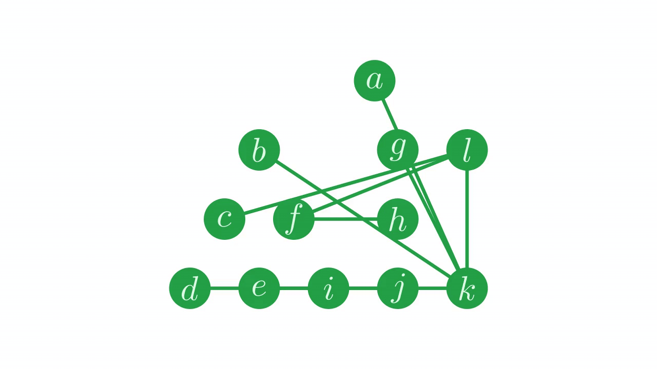
Fig. 14 Fixing the parent pointers.#
The result of this is a shuffled parent vector, with parent pointers set so as to represent exactly the same tree we started with.
Favourite Children (Ordering Siblings)#
Before we go any further, it’s worth making a note of the ordering requirements for a parent vector. We know that one of the big advantages of the representation is that it’s not constrained by the DFPT order, you can place parents and children in any order you like so long as each node points to its correct parent.
Sometimes, the order of siblings in a tree matters. Without any extra information, the only way to store the order of siblings in a tree is by their order in the parent vector. Throughout this tutorial, we’re going to use operations which maintain sibling ordering in the vast majority of cases, and we’ll be explicit where we don’t. The good news is, if your use of trees doesn’t require maintaining the order of siblings, you don’t have to worry about this at all!
Inverting#
Because it doesn’t really fit anywhere else in the tutorial, let’s look at a neat way to reverse the order of all siblings in a tree - in other words, mirroring the tree.
We will again reset our tree.
⊢p←parent
0 0 1 2 2 1 0 6 7 7 7 0
On our example tree, inverting looks like this:
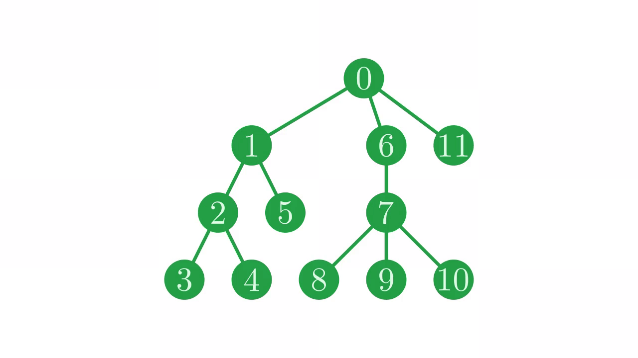
Fig. 15 Mirroring the tree.#
Our first step is to invert the parent vector is simply reverse it.
⌽p
0 7 7 7 6 0 1 2 2 1 0 0
Since the whole vector has been reversed, the order between siblings is reversed as well. Sadly, we’re not done. If a node i’s parent was j in the original p, that parent will now be in place ¯1+(≢p)-j - in our \(12\) element vector, node \(11\) goes to place \(0\), \(10\) goes to \(1\), and so on. Therefore, after reversing the parent vector, we can correct the parent pointers like so:
¯1+(≢p)-⌽p    ⍝ explicitly
(¯1+≢-⌽)p     ⍝ tacitly
11 4 4 4 5 11 10 9 9 10 11 11
11 4 4 4 5 11 10 9 9 10 11 11
Note that we could also have used the general method for fixing parents that we saw earlier, with ⌽⍳≢p as our permutation vector. The method we use here exploits the specific knowledge we have of how we shuffle the tree, and as a result is more performant than the general method for most tree sizes [1].
Pretty Printing#
We’re now looking at some sufficiently complicated tree operations that you might like to play around with other examples in the APL session yourself. It can be extremely frustrating to try an expression and be met just with a list of numbers and no way of visualising the resulting tree. For this reason, we’re going to include here some definitions that will let you pretty-print trees as character matrices, which you can copy and use right away. If you’re so inclined, you can have a crack at reading the code right away, but the general techniques it employs will be explained in due course.
Show code cell content
Depths←{ ⍝ find the depths of each node in a parent vector
    ⍝ ←: a vector of the depths of each node in the input
    p←⍵    ⍝ input parent vector
    depths←(≢p)⍴0
    StepUp←{ ⍝ step up the tree and increment depths
        q←p[⍵]
        depths+←⍵≠q
        q
    }
    _←StepUp⍣≡⍳≢p
    depths
}

_PrettyPrint_←{ ⍝ renders a tree given labels, box drawing characters, and padding
    ⍝ ←: vector of character matrices, each a labelled rendering of a tree in the forest given by the input parent vector
    labels    ←⍺     ⍝ vector of character matrices giving the labels for each node
    connectors←⍺⍺    ⍝ box drawing characters to render the tree, e.g: '─┌┬┐│┴├┼┤│' (normal, and upstruck)
    spaces    ←⍵⍵    ⍝ number of spaces to pad with between sub-trees
    p         ←⍵     ⍝ parent vector
    d←Depths p
    maxDepth←⌈/d
    results←labels         ⍝ result of rendering each sub-tree, seeded with labels
    maxDepth=0: results    ⍝ avoid the each running on the prototype
    DoFamily←{ ⍝ render and record a sub-tree
        ⍝ ⍺: parent node
        ⍝ ⍵: rendered results of children
        widths←(1⊃⍴)¨⍵                                                                           ⍝ widths of each rendered child
        width←spaces-⍨+/spaces+widths                                                            ⍝ eventual width of the rendered tree       wwwwwww
        centres←(+\0,¯1↓spaces+widths)+¯1+⌈2÷⍨widths                                             ⍝ centres of each rendered sub-tree         ∘ss∘ss∘
        result←width⍴' '                                                                         ⍝ header to be decorated                   '       '
        result[(⊢⊢⍤/⍨((⊃⌽centres)>⊢)∧(⊃centres)<⊢)⍳width]←connectors[0]                          ⍝ add horizontal bar                       ' ───── '
        result[   ⊃ centres]←connectors[1]                                                       ⍝ left end of bar                          '┌───── '
        result[   ⊃⌽centres]←connectors[3]                                                       ⍝ right end of bar                         '┌─────┐'
        result[¯1↓1↓centres]←connectors[2]                                                       ⍝ connectors to intermediate children      '┌──┬──┐'
        result[(1=≢centres)⍴⊃centres]←connectors[4]                                              ⍝ if there's only one child, just make it a lone upstrike
        centre←¯1+⌈2÷⍨width                                                                      ⍝ index of the centre of the rendered tree     ∘
        result[centre]←connectors[5 6 7 8 9][connectors[0 1 2 3 4]⍳result[centre]]               ⍝ connector to the parent                  '┌──┼──┐'
        result⍪←(-spaces)↓⍤1⊃,/,∘(spaces⍴' ')⍤1¨⍵↑¨⍨⌈/≢¨⍵                                        ⍝ pad lables, join under header
        parentResult←⍺⊃results                                                                   ⍝ label of the parent
        parentWidth←1⊃⍴parentResult                                                              ⍝ width of label of parent
        parentCentre←¯1+⌈2÷⍨parentWidth                                                          ⍝ centre of label of parent
        result      ←((centre-parentCentre)⌽parentWidth↑⍤1⊢)⍣(width<parentWidth)⊢result          ⍝ pad and recentre text so far if it's less wide
        parentResult←((parentCentre-centre)⌽      width↑⍤1⊢)⍣(width>parentWidth)⊢parentResult    ⍝ pad and recentre parent label if it's less wide
        result⍪⍨←parentResult                                                                    ⍝ add parent label
        results[⍺]←⊂result                                                                       ⍝ record result
        1
    }
    DoLayer←{ ⍝ render and record all nodes whose children have depth ⍵
        ⍝ ⍵: depth to handle nodes at
        i←⍸d=⍵    ⍝ nodes at this depth
        _←p[i]DoFamily⌸results[i]
        1
    }
    _←DoLayer¨⌽1+⍳maxDepth    ⍝ bottom up accumulation
    results/⍨p=⍳≢p            ⍝ return results at roots only
}

PPV←{⍺←'∘' ⋄   ((≢⍵)⍴⍉⍤⍪⍤⍕¨'∘'@(0=≢¨)⍺)('─┌┬┐│┴├┼┤│'_PrettyPrint_ 1)⍵}    ⍝ vertical
PPH←{⍺←'∘' ⋄ ⍉¨((≢⍵)⍴  ⍪⍤⍕¨'∘'@(0=≢¨)⍺)('│┌├└─┤┬┼┴─'_PrettyPrint_ 0)⍵}    ⍝ horizontal
(You may also find this essay by Roger Hui interesting.)
We now have access to the PPV and PPH functions to visualise trees both vertically and horizontally. These functions take a parent vector as their right argument, and optionally a scalar label or vector of labels as their left argument. The left argument is reshaped to the length of the given parent vector, and matched up so that node \(0\) used label \(0\), node \(1\) uses label \(1\), and so on.
PPV p ⍝ visualise vertically
┌─────────────┐
│      ∘      │
│  ┌───┴─┬───┐│
│  ∘     ∘   ∘│
│ ┌┴─┐   │    │
│ ∘  ∘   ∘    │
│┌┴┐   ┌─┼─┐  │
│∘ ∘   ∘ ∘ ∘  │
└─────────────┘
PPH p ⍝ visualise horizontally
┌───────┐
│   ┌∘┬∘│
│ ┌∘┤ └∘│
│ │ └∘  │
│∘┤   ┌∘│
│ ├∘─∘┼∘│
│ │   └∘│
│ └∘    │
└───────┘
'*' PPV p ⍝ change the label
┌─────────────┐
│      *      │
│  ┌───┴─┬───┐│
│  *     *   *│
│ ┌┴─┐   │    │
│ *  *   *    │
│┌┴┐   ┌─┼─┐  │
│* *   * * *  │
└─────────────┘
(⍳≢p) PPV p ⍝ label each node by its index
┌───────────────┐
│       0       │
│  ┌────┴┬────┐ │
│  1     6    11│
│ ┌┴─┐   │      │
│ 2  5   7      │
│┌┴┐   ┌─┼─┐    │
│3 4   8 9 10   │
└───────────────┘
This lets us check the results of the tree transformations we’ve done on this page:
⍝ children of nodes 1 and 6
i←1 6
(p∊i) PPV p
┌─────────────┐
│      0      │
│  ┌───┴─┬───┐│
│  0     0   0│
│ ┌┴─┐   │    │
│ 1  1   1    │
│┌┴┐   ┌─┼─┐  │
│0 0   0 0 0  │
└─────────────┘
⍝ leaf nodes
(~(⍳≢p)∊p) PPV p
┌─────────────┐
│      0      │
│  ┌───┴─┬───┐│
│  0     0   1│
│ ┌┴─┐   │    │
│ 0  1   0    │
│┌┴┐   ┌─┼─┐  │
│1 1   1 1 1  │
└─────────────┘
⍝ trimming branches
i←6
p[i]←i
(⍳≢p) PPV p
┌────────┬──────┐
│   0    │  6   │
│  ┌┴──┐ │  │   │
│  1   11│  7   │
│ ┌┴─┐   │┌─┼─┐ │
│ 2  5   │8 9 10│
│┌┴┐     │      │
│3 4     │      │
└────────┴──────┘
Note that the output of PPV is a vector of character matrices, one for each tree represented in the parent vector.
⍝ finding roots
(I⍣≡⍨p) PPV p
┌───────┬─────┐
│   0   │  6  │
│  ┌┴──┐│  │  │
│  0   0│  6  │
│ ┌┴─┐  │┌─┼─┐│
│ 0  0  │6 6 6│
│┌┴┐    │     │
│0 0    │     │
└───────┴─────┘
⍝ selecting sub-trees
p←parent
i←1 6
(i∊⍨p I@{~⍵∊i}⍣≡⍳≢p) PPV p
┌─────────────┐
│      0      │
│  ┌───┴─┬───┐│
│  1     1   0│
│ ┌┴─┐   │    │
│ 1  1   1    │
│┌┴┐   ┌─┼─┐  │
│1 1   1 1 1  │
└─────────────┘
⍝ mirroring
(⌽⍳≢p) PPV (¯1+≢-⌽)p
┌───────────────┐
│       0       │
│┌────┬─┴────┐  │
│11   6      1  │
│     │    ┌─┴┐ │
│     7    5  2 │
│   ┌─┴┬─┐   ┌┴┐│
│   10 9 8   4 3│
└───────────────┘