Relating the Depth and Parent Vectors#
While we are focusing on the parent vector representation, the depth vector is still very useful, and in many applications we will begin with a depth vector and later construct a parent vector. This page covers constructing a parent vector from a depth vector, finding the depths of nodes in a parent vector, and ordering a parent vector in the same way as the corresponding depth vector.
Constructing the Parent Vector#
The first thing we’ll look at is constructing a parent vector, given a depth vector. In the page on working with ⎕JSON, we will begin with a depth vector, and construct a parent vector in order to do more complicated operations. So it’s important for us to be able to make this conversion.
Let’s look at the same tree we worked with in the page on representing trees.
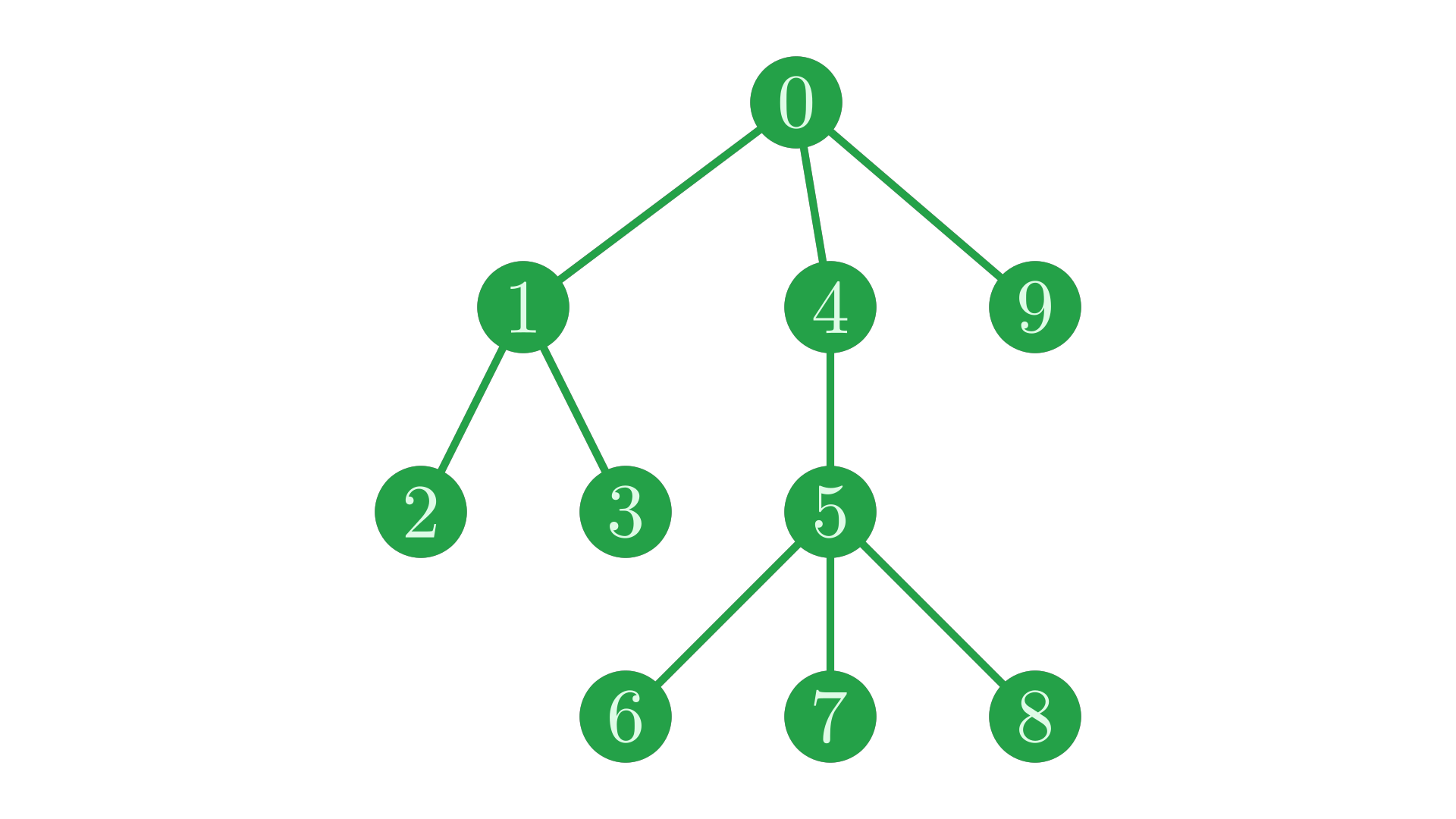
Fig. 16 Our simple tree.#
The depth vector for this tree is:
d←0 1 2 2 1 2 3 3 3 1
For each node i in this tree, we want to find the index j of the node which is the parent of i. Recall that the nodes in any sub-tree are necessarily adjacent in the depth vector. Also notice that the root of a sub-tree appears immediately before all of its descendents.
Fig. 17 The location of a sub-tree in the depth vector.#
Finally, if j is the parent of i, we know that j must have a depth one less than the depth of i, i.e. d[j]=d[i]-1. All of this information together leads to a neat method for constructing a parent vector from a depth vector.
Firstly, we want to group the nodes in the depth vector by their given depth. ⌸ (Key) is the perfect primitive for this:
⊂⍤⊢⌸d
┌─┬─────┬─────┬─────┐
│0│1 4 9│2 3 5│6 7 8│
└─┴─────┴─────┴─────┘
Here, we have grouped the nodes in the tree by their depth. ⌸ orders the groups it creates by the order the values appear in its right argument. The ordering of the depth vector ensures that this is exactly the all of the possible depths of the tree in ascending order. So, at index \(0\) we have all nodes with a depth of \(0\) (in our case just the single root), at index \(1\) we have all those with a depth of \(1\), and so on.
Any non-root node i will appear after its parent j in the depth vector, and before the next node at the same depth as its parent. It is not possible for there to be another node with the same depth as j which appears between i and j.
   no 1s here
      ┌┴┐
d: 0 1 2 2 1 2 3 3 3 1
     ↑   ↑
     j   i
Look again at our nodes grouped by their depth:
⊂⍤⊢⌸d
┌─┬─────┬─────┬─────┐
│0│1 4 9│2 3 5│6 7 8│
└─┴─────┴─────┴─────┘
Since the parent of i has depth one less than i, it must appear in the group immediately preceding the group that contains i. Within that group, the parent of i must be the leftmost node (i.e. node with the largest index) that is not later than (has a greater index than) i. In this sense, the groups define intervals of the indexes of the depth vector, splitting it up into sub-trees. We can use this to find the parent of each node using ⍸ (Interval Index).
i←3               ⍝ let's find the parent of node 3
1 4 9⍸i           ⍝ where in the group is the parent of node 3
1 4 9[1 4 9⍸i]    ⍝ which node is the parent of node 3
0
1
Of course, this works for finding the parents of the whole group of nodes at a certain depth.
i←2 3 5           ⍝ all nodes at depth 2
1 4 9⍸i
1 4 9[1 4 9⍸i]
0 0 1
1 1 4
We can use this trick to finally construct the parent vector corresponding to the tree. First we initialise the parent vector so that all nodes are roots. We will update all non-roots with their parents.
⊢p←⍳≢d
0 1 2 3 4 5 6 7 8 9
We then want to look at each adjacent pair of groups and update p accordingly, which we can do with a windowed reduction:
⍝  ┌──┬─ {⍺⍵} is executed with ⍺ as the left group and ⍵ as the right group
  2{⍺⍵}/⊂⍤⊢⌸d
  2{p[⍵]←⍺[⍺⍸⍵]}/⊂⍤⊢⌸d
⍝  └───────────┴─ instead, we can use our method to update p
┌─────────┬─────────────┬─────────────┐
│┌─┬─────┐│┌─────┬─────┐│┌─────┬─────┐│
││0│1 4 9│││1 4 9│2 3 5│││2 3 5│6 7 8││
│└─┴─────┘│└─────┴─────┘│└─────┴─────┘│
└─────────┴─────────────┴─────────────┘
After this operation, we have successfully created the parent vector corresponding to d.
p
d PPV p
0 0 1 1 0 4 5 5 5 0
┌───────────┐
│     0     │
│ ┌───┴┬───┐│
│ 1    1   1│
│┌┴┐   │    │
│2 2   2    │
│    ┌─┼─┐  │
│    3 3 3  │
└───────────┘
Putting it all together:
DepthToParent←{ ⍝ return the parent vector representation of a tree from a depth vector
    ⍝ ←: the parent vector corresponding to the depth vector input
    d←⍵                       ⍝ depth vector to be parentified
    p←⍳≢d                     ⍝ begin by setting all nodes as roots
    _←2{p[⍵]←⍺[⍺⍸⍵]}/⊂⍤⊢⌸d    ⍝ find the parents of each non-root
    ⍝ │ │   ││    │ │└───┴─ indices of each level
    ⍝ └─│───││────│─┴─ pairwise between levels
    ⍝   │   │└────┴─ leftmost node at previous level - the parent
    ⍝   └───┴─ make this the parent
    p
}
Now that we can convert depth vectors to parent vectors, a natural next question is converting parent vectors back into depth vectors. There are two stages to this: firstly finding the depths of each node, and secondly imposing the DFPT ordering on the nodes.
Recovering Depths#
We will look at finding the depths of each node in a parent vector first. Our method will be roughly to see how many jumps to parents it takes to reach a root.
Take our current tree:
(⍳≢p) PPV p
┌───────────┐
│     0     │
│ ┌───┴┬───┐│
│ 1    4   9│
│┌┴┐   │    │
│2 3   5    │
│    ┌─┼─┐  │
│    6 7 8  │
└───────────┘
Since we constructed this parent vector from a depth vector, it is already in DFPT order. To emphasise that the parent vector need not be in this order (and to give us something to do when we get the order back), we’re going to shuffle it.
perm←3 5 1 7 0 6 8 2 4 9    ⍝ an arbitrary(-ish) permutation of the nodes
⊢p←perm⍳p[perm]
(⍳≢p) PPV p
2 8 4 1 4 1 1 2 4 4
┌───────────┐
│     4     │
│ ┌───┴┬───┐│
│ 2    8   9│
│┌┴┐   │    │
│0 7   1    │
│    ┌─┼─┐  │
│    3 5 6  │
└───────────┘
Note that the particular shuffle we’ve chosen here preserves the order of siblings in the tree. If your use of trees depends on sibling order, you’ll want to make sure that any time your tree is re-ordered, the order of siblings is preserved.
To find the depth of each of these nodes, we will repeatedly follow parent pointers until we reach a root. Once we do reach a root, the number of jumps it took to get there will be the depth of the node.
Let’s use node \(1\) as an example. This node has depth \(2\), which we can be sure of as two parental jumps reaches a root.
p[1]          ⍝ depth ≥ 1 since 1 is not a root
p[p[1]]       ⍝ depth ≥ 2 since p[1] is not a root
p[p[p[1]]]    ⍝ depth = 2 since p[p[1]] is a root
8
4
4
Since we’re traversing the tree until the parent does not change, we can automate this repetition with ⍣≡ to find the depth of any particular node.
depth←0           ⍝ seed value
StepUp←{
    q←p[⍵]        ⍝ parent of current node
    depth+←⍵≠q    ⍝ increment depth if not a root
    q
}
_←StepUp⍣≡1
depth             ⍝ node 1 has depth 2
2
This method can be easily extended to find the depths of all nodes at once.
depths←(≢p)⍴0      ⍝ seed for all nodes
StepUp←{
    q←p[⍵]
    depths+←⍵≠q    ⍝ increment for each path which has not hit a root
    q
}
_←StepUp⍣≡⍳≢p        ⍝ all nodes this time
depths
depths PPV p
2 2 1 3 0 3 3 2 1 1
┌───────────┐
│     0     │
│ ┌───┴┬───┐│
│ 1    1   1│
│┌┴┐   │    │
│2 2   2    │
│    ┌─┼─┐  │
│    3 3 3  │
└───────────┘
Wrapping it all up in a dfn:
Depths←{ ⍝ find the depths of each node in a parent vector
    ⍝ ←: a vector of the depths of each node in the input
    p←⍵    ⍝ input parent vector
    depths←(≢p)⍴0
    StepUp←{ ⍝ step up the tree and increment depths
        q←p[⍵]
        depths+←⍵≠q
        q
    }
    _←StepUp⍣≡⍳≢p
    depths
}
(Depths p) PPV p
┌───────────┐
│     0     │
│ ┌───┴┬───┐│
│ 1    1   1│
│┌┴┐   │    │
│2 2   2    │
│    ┌─┼─┐  │
│    3 3 3  │
└───────────┘
Remember: depths is not in DFPT order! Our next task will be to put it back in that order to fully recover the depth vector.
Challenge: Can you change the initial conditions of our method so that we can skip the first iteration?
Solution:
Show code cell content
Depths←{ ⍝ find the depths of each node in a parent vector
    p←⍵
    depths←p≠⍳≢p    ⍝ skip the first iteration by incrementing non-roots up-front
    StepUp←{
        q←p[⍵]
        depths+←⍵≠q
        q
    }
    _←StepUp⍣≡p     ⍝ we can now skip straight to p
    depths
}
(Depths p) PPV p
┌───────────┐
│     0     │
│ ┌───┴┬───┐│
│ 1    1   1│
│┌┴┐   │    │
│2 2   2    │
│    ┌─┼─┐  │
│    3 3 3  │
└───────────┘
Depth Vector Ordering#
Having recovered the depths of each node, the next step fully reconstructing the depth vector for a tree is imposing the DFPT ordering. To do this, we’re going to augment our method for find depths to build up a kind of path matrix for the tree as we go. We can then use the paths to find the DFPT ordering.
To begin with, let’s initialise an empty matrix.
paths←(≢p)0⍴⍬
Now, as we traverse the tree to find depths, we can also record the ancestors found at each iteration into paths.
depths←(≢p)⍴0
StepUp←{
    paths,←⍵       ⍝ record the nodes found at this iteration
    q←p[⍵]
    depths+←⍵≠q
    q
}
_←StepUp⍣≡⍳≢p
Now, if we look at paths, we can see that the first column is all the nodes in the tree, the second column is their parents, and so on.
paths
0 2 4 4
1 8 4 4
2 4 4 4
3 1 8 4
4 4 4 4
5 1 8 4
6 1 8 4
7 2 4 4
8 4 4 4
9 4 4 4
Each row records a path from node to root, with padding at the end for shallow nodes. We a little effort, we can extract the paths from root to node, without padding.
⍪paths←⌽¨(depths+1)⊂⍤↑⍤¯1⊢paths
⍝      ││└───────────┴─ there are depths[i]+1 nodes on the path from i to the root
⍝      └┴────────────── get root → node rather than node → root
┌───────┐
│4 2 0  │
├───────┤
│4 8 1  │
├───────┤
│4 2    │
├───────┤
│4 8 1 3│
├───────┤
│4      │
├───────┤
│4 8 1 5│
├───────┤
│4 8 1 6│
├───────┤
│4 2 7  │
├───────┤
│4 8    │
├───────┤
│4 9    │
└───────┘
If we look again at our tree, and list out the first few paths in the DFPT of it, we notice an interesting pattern.
(⍳≢p) PPV p
┌───────────┐
│     4     │
│ ┌───┴┬───┐│
│ 2    8   9│
│┌┴┐   │    │
│0 7   1    │
│    ┌─┼─┐  │
│    3 5 6  │
└───────────┘
4
4 → 2
4 → 2 → 0
4 → 2 → 7
4 → 8
4 → 8 → 1
...
In the DFPT, the paths are ordered first by the size of the index in each place (\(0<7\), \(2<8\), etc), and then by the length of the whole paths. This is exacly a lexicographic ordering of the paths. Fortunately for us, this is also the ordering which ⍋ uses to grade arrays. Therefore, finding the DFPT order of the nodes is as simple as ⍋ing the paths.
⍪paths[⍋paths]
┌───────┐
│4      │
├───────┤
│4 2    │
├───────┤
│4 2 0  │
├───────┤
│4 2 7  │
├───────┤
│4 8    │
├───────┤
│4 8 1  │
├───────┤
│4 8 1 3│
├───────┤
│4 8 1 5│
├───────┤
│4 8 1 6│
├───────┤
│4 9    │
└───────┘
Using this order to rearrange the depths of the nodes gives us exactly the depth vector for our tree.
depths[⍋paths]
0 1 2 2 1 2 3 3 3 1
Huzzah! This is the depth vector we started with at the top of the page.
As we’ll see later, we often have other vectors of data associated with our trees. When we find the depth vector of a tree, we will also want to re-order this extra data so that it still lines up. Therefore, when we wrap this method up in a dfn, we will have it return the depths and the ordering separetely, allowing the caller to use the ordering to shuffle any extra data they like.
ParentToDepth←{ ⍝ recover the depths and DFPT ordering of a parent vector
    ⍝ ←: a two element vector consisting of (1) the depths of each node and (2) the permutation vector for DFPT order
    p←⍵    ⍝ input parent vector
    paths←(≢p)0⍴⍬
    depths←(≢p)⍴0
    StepUp←{
        paths,←⍵
        q←p[⍵]
        depths+←⍵≠q
        q
    }
    _←StepUp⍣≡⍳≢p
    order←⍋⌽¨(depths+1)⊂⍤↑⍤¯1⊢paths
    depths order
}