Representing Trees

In this section, we’re going to look at several different ways to represent trees as arrays, and we’re going to settle on one as the main representation we’ll be looking at for the rest of the tutorial.

Preliminary Definitions

Before we go any further, let’s nail down one thing.

⎕IO←0

The unending debate over what value ⎕IO should take rages on. I don’t have a particular favourite, but we just need to pick one and be consistent with it throughout our study of trees.

Additionally, there are some places where we’re going to want to use indexing functionally, so it will be helpful to define:

I←{⍺[⍵]}

If/when Dyalog gets the proposed Select function, we’ll be able to drop the name and just write ⊇⍨, but for now we will use I.

Finally, for cosmetic reasons:

]box on

Was OFF

The Nested Representation

The naive way to represent a tree with an array is with a nested vector. Each node in a tree has an associated piece of data and some number of child nodes. We can represent this structure directly in a nested vector by storing the data of each node as the first element, and then storing the nested vectors representing the child nodes in the tail of the vector.

Take the simple tree from the previous page:

Fig. 2 A simple tree.

We can represent this tree like so:

(,'a') ((,'b') (,⊂,'e') (,⊂,'f')) ((,'c') ((,'g') (,⊂,'h') (,⊂,'i') (,⊂,'j'))) (,'d')

┌─┬───────────┬───────────────────┬─┐
│a│┌─┬───┬───┐│┌─┬───────────────┐│d│
│ ││b│┌─┐│┌─┐│││c│┌─┬───┬───┬───┐││ │
│ ││ ││e│││f││││ ││g│┌─┐│┌─┐│┌─┐│││ │
│ ││ │└─┘│└─┘│││ ││ ││h│││i│││j││││ │
│ │└─┴───┴───┘││ ││ │└─┘│└─┘│└─┘│││ │
│ │           ││ │└─┴───┴───┴───┘││ │
│ │           │└─┴───────────────┘│ │
└─┴───────────┴───────────────────┴─┘

The vector represents the root node labelled a, with the label stored as the first element, and the representations of the children placed in the tail.

While messy to write out, this representation is elegant, and in most programming paradigms this kind of representation is used for working with trees. However, this structure isn’t suited for making the most of APL. To get really good performance, it’s important for us to be working with flat arrays. Deeply nested arrays are stored internally with pointers to potentially disparate allocations in the workspace. Traversing these pointers is a costly operation, compared to using APL’s well optimised array primitives.

The Depth Vector Representation

So, let’s try to find a more APL-friendly representation for trees. Some information that tells us a lot about the structure of a tree is the depth of each node. We say the root node of a tree has depth \(0\), the root’s children have depth \(1\), their children have depth \(2\), and so on.

We can label each node of our example tree with its depth:

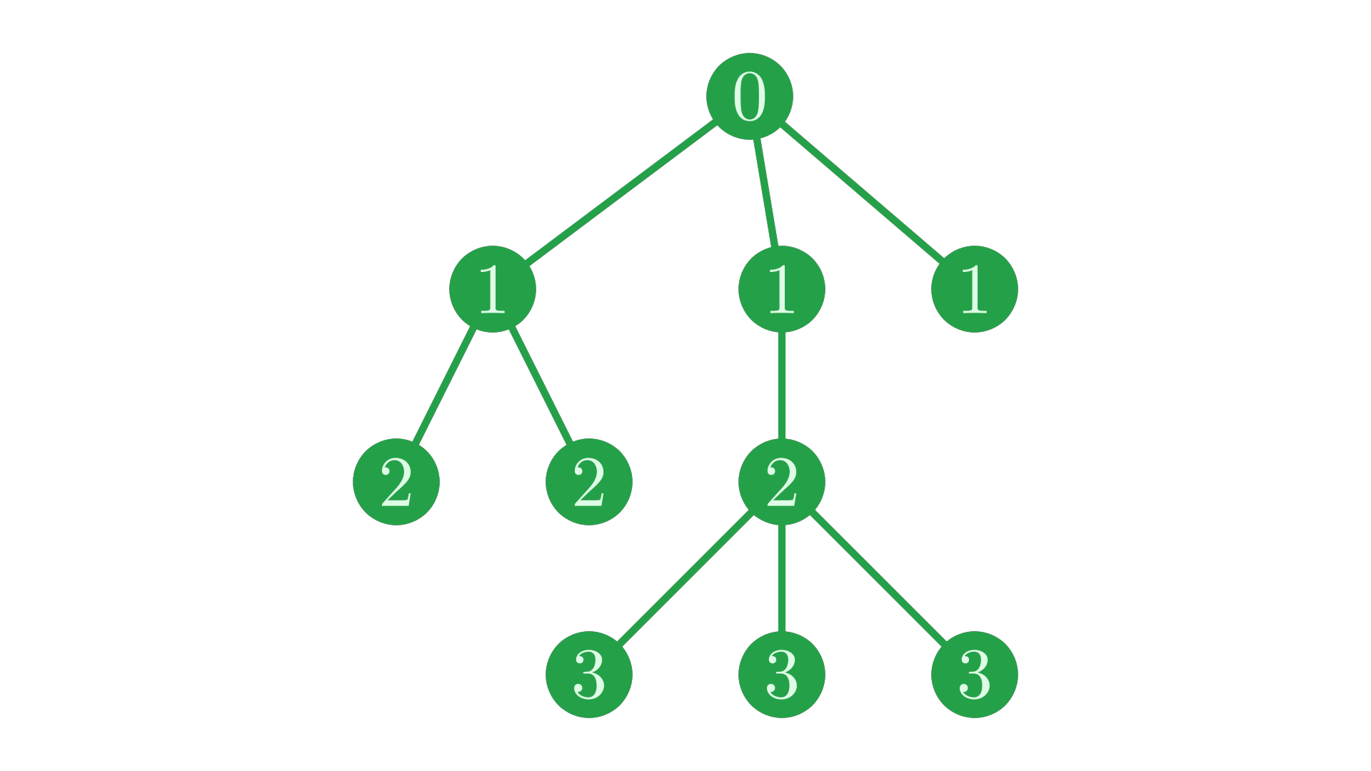
Fig. 3 The same tree, with nodes labelled with their depth.

Notice that the depth corresponds to horizontal levels in the tree, and that siblings share the same depth.

It’s fairly straightforward to calculate the depth of each node for a tree represented by a nested vector:

t←(,'a') ((,'b') (,⊂,'e') (,⊂,'f')) ((,'c') ((,'g') (,⊂,'h') (,⊂,'i') (,⊂,'j'))) (,'d')
NestedDepth←{
    ⍺←0
    ⍝ ⍵: nested vector corresponding to a sub-tree
    ⍝ ⍺: depth of the sub-tree (0 at the root)
    1=≢⍵: ,⍺        ⍝ if there are no children, just return own depth
    ⍺,(⍺+1)∇¨1↓⍵    ⍝ else, recursively find depths of children
}
NestedDepth t

┌─┬───────┬─────────────┬─┐
│0│┌─┬─┬─┐│┌─┬─────────┐│1│
│ ││1│2│2│││1│┌─┬─┬─┬─┐││ │
│ │└─┴─┴─┘││ ││2│3│3│3│││ │
│ │       ││ │└─┴─┴─┴─┘││ │
│ │       │└─┴─────────┘│ │
└─┴───────┴─────────────┴─┘

Reading this result from left to right (0, 1, 2, 2, 1, and so on), we can see some useful patterns. Every time the depth steps up by one, we are descending to a child node. Similarly, whenever the depth decreases, we are ascending to a sibling of an ancestor. This means that we can do away with the nesting, keeping only the depth numbers, and preserve a full description of the structure of the tree.

⊢depths←∊NestedDepth t

0 1 2 2 1 2 3 3 3 1

We call this description of a tree a depth vector. Nodes are now identified by an index into this vector. On its own, the depth vector doesn’t tell us anything about the extra data associated with each node. We therefore need to store the data associated with each node in a separate vector.

⊢data←,¨'abefcghijd'

┌─┬─┬─┬─┬─┬─┬─┬─┬─┬─┐
│a│b│e│f│c│g│h│i│j│d│
└─┴─┴─┴─┴─┴─┴─┴─┴─┴─┘

The data vector is indexed by the same indices as the depths vector, so that for a node at index i, depths[i] is its depth and data[i] is its data.

↑(⊂¨'index:' 'depths:' 'data:'),¨(⍳≢depths) depths data

┌───────┬─┬─┬─┬─┬─┬─┬─┬─┬─┬─┐
│index: │0│1│2│3│4│5│6│7│8│9│
├───────┼─┼─┼─┼─┼─┼─┼─┼─┼─┼─┤
│depths:│0│1│2│2│1│2│3│3│3│1│
├───────┼─┼─┼─┼─┼─┼─┼─┼─┼─┼─┤
│data:  │a│b│e│f│c│g│h│i│j│d│
└───────┴─┴─┴─┴─┴─┴─┴─┴─┴─┴─┘

At this point it’s helpful to make a small mental shift. We are drawing a one-to-one correspondence between node and indices into these vectors, using the indices as unique identifiers. We will use this so frequently that making the distinction explicit becomes tiring, so from now on, we will often refer to ‘the node associated with index i’ simply as ‘node i’.

Labelling each node of our tree with its corresponding index reveals an interesting pattern.

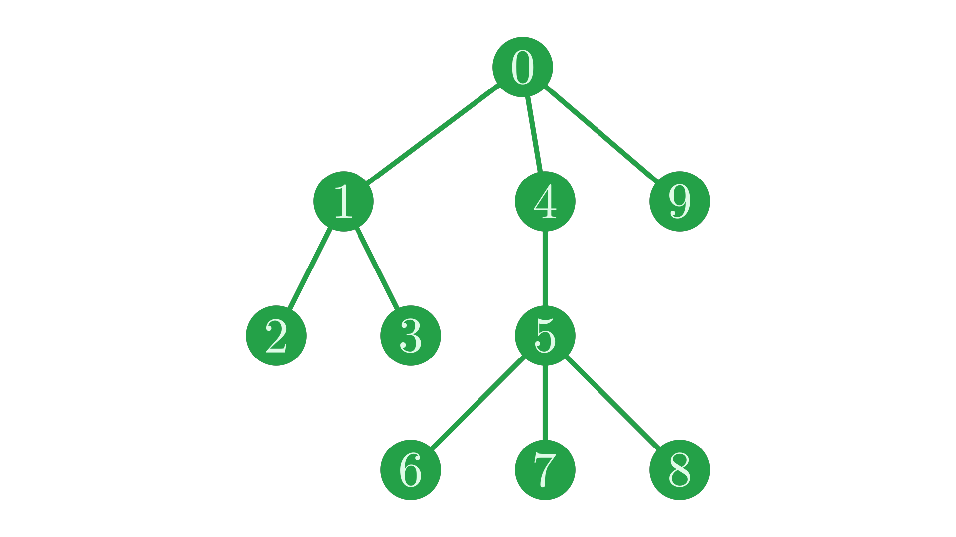
Fig. 4 The same tree, with nodes labelled with their index into the depth and data vectors.

If we trace the path through the tree given by these indices, we find that we traverse the tree in a particular pattern. We dive down the tree until we hit a leaf node (\(0 \to 1 \to 2\)). When we reach a leaf node, we step back along our path until we find a junction with an unexplored path, and then resume our traversal, once again descending until we hit a leaf before backtracking. In technical jargon, this is a depth-first, pre-order traversal (or DFPT).

Fig. 5 The depth-first, pre-order traversal in action.

So the depth vector representation orders nodes exactly in a DFPT ordering. This presents a problem for manipulating trees in this format, as we are required to maintain this ordering exactly whenever we change the structure of the tree, which can be fairly inconvenient and costly. Especially, we would like to be able to append data to the end of the depth vector when adding nodes, as this is implemented more efficiently in the Dyalog interpreter than splicing into the middle of the vector, but the ordering requirements forbid us from doing this in most cases.

Additionally, we often want to find parents or siblings of a node for various reasons. In the depth vector, sub-trees are stored contiguously.

Fig. 6 The location of a sub-tree in the depth vector.

This structure means that, given a node i, finding the parent and siblings of i requires linearly scanning through the depth vector forwards and backwards from i to find places with the correct depth, which can become extremely costly on large vectors when sub-trees take up lots of space.

               siblings of i
                   ┌─┴─┐
depth: 0 1 2 2 1 2 3 3 3 1
                 ↑   ↑   ↑
    parent of i ─┘   i   └─ start of next sub-tree

The depth vector representation is therefore only useful in some situations. Indeed, we’ll find it very handy in the page on working with ⎕JSON, but it is not the representation that we would like to settle on for most of our operations.

The Path Matrix Representation

Take another look at that animation of the depth-first pre-order traversal, and notice that each node is visited on a unique path from the root. Let’s write out these paths, indicating nodes by their index into the depth vector.

⍪paths←(,0)(0 1)(0 1 2)(0 1 3)(0 4)(0 4 5)(0 4 5 6)(0 4 5 7)(0 4 5 8)(0 9)

┌───────┐
│0      │
├───────┤
│0 1    │
├───────┤
│0 1 2  │
├───────┤
│0 1 3  │
├───────┤
│0 4    │
├───────┤
│0 4 5  │
├───────┤
│0 4 5 6│
├───────┤
│0 4 5 7│
├───────┤
│0 4 5 8│
├───────┤
│0 9    │
└───────┘

We can make this representation more compact by mixing the vectors and simply repeating node IDs to fill in the gaps.

⊢pathMatrix←⌈\↑paths

0 0 0 0
0 1 1 1
0 1 2 2
0 1 3 3
0 4 4 4
0 4 5 5
0 4 5 6
0 4 5 7
0 4 5 8
0 9 9 9

We call this format the path matrix representation of a tree. Each ith row of this matrix gives the path to node i, but notice that the ordering of the nodes are no longer constrained as they were in the depth vector representation - the ancestry of a node is stored directly, so we no longer need to implicitly encode it in the node ordering.

This means that, as long as the indices in the matrix are adjusted accordingly, we can shuffle the rows arbitrarily and maintain the same tree structure.

perm←3 6 8 0 2 7 1 5 9 4    ⍝ some arbitrary permutation of the nodes
perm⍳pathMatrix[perm;]      ⍝ permute the matrix and update the indices

3 6 0 0
3 9 7 1
3 9 7 2
3 3 3 3
3 6 4 4
3 9 7 5
3 6 6 6
3 9 7 7
3 8 8 8
3 9 9 9

This path matrix represents exactly the same tree structure, with the node identifiers permuted:

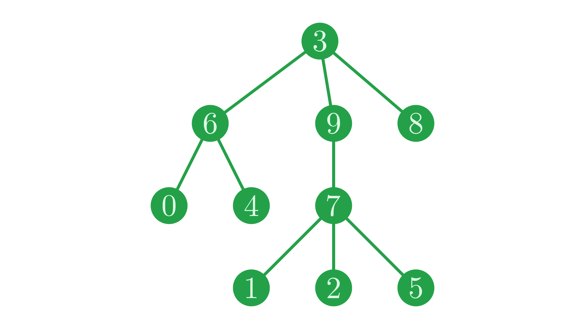
Fig. 7 Our tree with labels permuted.

These nice properties and others would make the path matrix representation ideal to work with, if it were not for one major downside: the space usage. Given a tree with \(n\) nodes and a maximum depth of \(d\), to fully encode the structure of this tree the depth vector representation only requires enough memory to store \(n\) depth numbers. The path matrix, on the other hand, requires \(n×d\) numbers, encoding the entire path for each node in the tree. For large trees, especially deep trees, this will use large amounts of memory and slow everything down.

The depth vector and path matrix representations are both not quite what we want, so we need to find some kind of compromise between their benefits.

The Parent Vector Representation

By focusing on the ancestry of nodes, the path matrix representation is more flexible than the depth vector representation, but by encoding more information implicitly, the depth vector representation is more space efficient. The compromise between these two approaches is the parent vector representation. For each node, instead of storing the entire path from the root as the path matrix does, the parent vector stores only the node’s immediate parent. For an example, take the same tree we’ve been examining throughout this section, identified once again with DFPT indices:

Fig. 8 Our favourite tree, back again.

The parent vector for this tree is:

⊢parent←0 0 1 1 0 4 5 5 5 0

0 0 1 1 0 4 5 5 5 0

Node \(2\) is a child of node \(1\), so parent[2]←1, \(1\) is a child of \(0\), so parent[1]←0, and so on. Each node ‘points to’ its parent.

        ┌─┐─────┐ ┌─┐─┐─┐
        ↓ │     │ ↓ │ │ │
parent: 0 0 1 1 0 4 5 5 5 0
        ↑ ↑ │ │ ↑ │       │
        │ └─┘─┘ └─┘       │
        └─────────────────┘

Following these pointers from any starting node will trace out the path to that node from the root, as found in the path matrix.

Notice that node \(0\), as the root, has no parent. We could use some kind of sentinel value like \(-1\) to indicate that a node has no parent. For reasons which will become clear as we work with this representation more, we instead have the root, node \(0\), point to itself.

Like the depth vector, the parent vector is extremely space efficient. Like the path matrix, it is not heavily constrained by ordering requirements. The nodes can be shuffled arbitrarily, so long as we update the parents in each place to reflect the shuffling.

This representation is suitable for most of our purposes, and it is the one we will focus on for the rest of the tutorial.

Challenge

Challenge: To make sure you really understand each of these representations, draw yourself a small tree on paper, and then write out the depth vector, path matrix, and parent vector for that tree. As you figure these out, you will get an idea of what the APL interpreter is spending its time doing when working with these representations.